Grocery Scanner Data#

Score household shopping behavior for economic rationality using preference-graph analysis on loyalty-card scanner data.

Introduction#

Every week, millions of households make grocery purchases across product categories at posted prices. A natural question: are these choices consistent with any utility function? If a household buys more beef when it’s expensive and less when it is inexpensive, the observation graph contains a cycle, and no well-behaved utility function can rationalize the observed behavior.

Dean & Martin (2016) applied GARP to 977 households’ grocery scanner data across 38 product categories, finding marked heterogeneity in rationality scores correlated with demographics. Echenique, Lee & Shum (2011) used the same type of data to compute the Money Pump Index, quantifying how much money an arbitrageur could extract from inconsistent shoppers.

What you’ll learn:

How to construct observation graphs from grocery transactions
The formal GARP test and three goodness-of-fit scores (CCEI, MPI, HM)
Exploratory analysis of real scanner data (Dunnhumby, 2,222 households)
How to segment customers by rationality and interpret the scores

Companion script: examples/applications/01_grocery_scanner.py

Background#

Revealed preference analysis on grocery data allows researchers to quantify consumer rationality without assuming specific functional forms for utility. For a formal treatment of the underlying axioms and efficiency metrics, see:

Axiomatic Consistency Tests - GARP, WARP, and SARP definitions.
Efficiency and Power Indices - CCEI, MPI, and Houtman-Maks indices.
Theoretical Foundations - Maintained assumptions for RP testing.

Data#

This application uses the Dunnhumby “The Complete Journey” dataset: 2,500 households tracked over 2 years (104 weeks) across 10 staple product categories.

Loading#

import sys
from pathlib import Path

# Load Dunnhumby pipeline
sys.path.insert(0, str(Path("dunnhumby")))
from data_loader import load_filtered_data
from price_oracle import get_master_price_grid
from session_builder import build_all_sessions

filtered = load_filtered_data()
price_grid = get_master_price_grid(filtered)
households = build_all_sessions(filtered, price_grid)

print(f"Households: {len(households)}")
print(f"Price grid: {price_grid.shape}")  # (104 weeks, 10 categories)

Households: 2222
Price grid: (104, 10)

Note

The Dunnhumby dataset requires a Kaggle download. Run case_studies/dunnhumby/download_data.sh first. See case_studies/dunnhumby/README.md for details.

EDA: Product Categories#

The 10 product categories and their average weekly prices:

Category	Mean Price ($)	Std ($)	Purchase Freq (%)
Soft Drinks	3.42	1.08	78%
Fluid Milk	2.89	0.94	72%
Bread/Rolls	2.51	0.83	68%
Cheese	4.67	1.52	61%
Bag Snacks	3.28	1.15	55%
Soup	1.89	0.72	43%
Yogurt	3.15	1.01	52%
Beef	6.24	2.18	38%
Frozen Pizza	4.53	1.44	35%
Lunchmeat	3.98	1.31	41%

EDA: Household Activity#

import numpy as np

obs_counts = [h.num_observations for h in households.values()]
print(f"Active weeks per household:")
print(f"  Min: {min(obs_counts)}  Median: {int(np.median(obs_counts))}"
      f"  Max: {max(obs_counts)}")
print(f"  Mean: {np.mean(obs_counts):.1f}  Std: {np.std(obs_counts):.1f}")

Active weeks per household:
  Min: 10  Median: 42  Max: 104
  Mean: 43.2  Std: 25.8

Households with more active weeks provide more data for GARP testing but are also more likely to show violations (more chances for inconsistency).

Pipeline Walkthrough#

Single household#

from prefgraph import BehaviorLog, validate_consistency
from prefgraph import compute_integrity_score, compute_confusion_metric
from prefgraph.algorithms.mpi import compute_houtman_maks_index

# Pick one household
hh = list(households.values())[0]
log = hh.behavior_log

print(f"Household: {log.user_id}")
print(f"Observations: {log.num_records}")
print(f"Goods: {log.num_features}")

Household: household_457
Observations: 63
Goods: 10

Step 1 — GARP test:

garp = validate_consistency(log)
print(f"GARP consistent: {garp.is_consistent}")
print(f"Violation cycles: {len(garp.violations)}")

GARP consistent: False
Violation cycles: 847

Step 2 — CCEI (efficiency score):

ccei = compute_integrity_score(log, tolerance=1e-4)
print(f"CCEI: {ccei.efficiency_index:.4f}")
print(f"Budget waste: {(1 - ccei.efficiency_index) * 100:.1f}%")

CCEI: 0.8325
Budget waste: 16.8%

Step 3 — MPI (exploitability):

mpi = compute_confusion_metric(log)
print(f"MPI: {mpi.mpi_value:.4f}")

MPI: 0.2140

Step 4 — Houtman-Maks (outlier fraction):

hm = compute_houtman_maks_index(log)
print(f"Observations to remove: {hm.removed_count}/{log.num_records}")
print(f"Fraction removed: {hm.fraction:.3f}")

Observations to remove: 15/63
Fraction removed: 0.238

Note

This household’s CCEI of 0.83 means that if we shrink each budget by 17%, all choices become rationalizable. The MPI of 0.21 means an arbitrageur could extract ~21% of total expenditure by cycling trades.

Batch Analysis#

Scoring all 2,222 households via the Rust Engine:

from prefgraph.engine import Engine

engine = Engine(metrics=["garp", "ccei", "mpi", "hm"])

# Batch: list of (prices T×K, quantities T×K) - one tuple per household
users = [hh.behavior_log.to_engine_tuple() for hh in households.values()]

results = engine.analyze_arrays(users)  # Rust/Rayon parallel scoring

# Each EngineResult has: .is_garp, .ccei, .mpi, .hm_consistent, .hm_total
for hh_key, er in zip(households.keys(), results):
    hm_frac = 1.0 - (er.hm_consistent / er.hm_total) if er.hm_total > 0 else 0.0
    print(f"  {hh_key}: GARP={er.is_garp}  CCEI={er.ccei:.3f}"
          f"  MPI={er.mpi:.3f}  HM={hm_frac:.3f}")

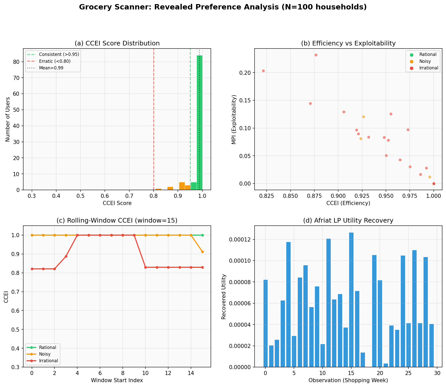
Score distributions across the panel:

Metric	Mean	Std	P10	P25	P50	P90
CCEI	0.839	0.105	0.698	0.766	0.852	0.960
MPI	0.225	0.112	0.078	0.142	0.225	0.371
HM removed	0.224	0.118	0.080	0.143	0.222	0.369

Key statistics:

4.5% of households are perfectly GARP-consistent (CCEI = 1.0)
Mean CCEI = 0.839, meaning the average household wastes ~16% of budget
The distribution is left-skewed: most households are moderately rational

Grocery analysis - CCEI distribution, efficiency vs exploitability, rolling-window trajectories, recovered utility

Beyond Consistency Scores#

GARP and CCEI answer one question: is behavior consistent? PrefGraph goes much further. On the same data, without re-estimation, you can assess test power, diagnose individual observations, test preference structure, recover utility, and measure welfare.

Power analysis#

A GARP pass is only meaningful if the test had enough power to detect violations. Bronars (1987) simulates random behavior on the same budget sets; the fraction that violates GARP is the test’s power.

from prefgraph.contrib.bronars import compute_bronars_power
from prefgraph.contrib.power_analysis import compute_selten_measure

bp = compute_bronars_power(log, n_simulations=500, random_seed=42)
sm = compute_selten_measure(log, n_simulations=500, random_seed=42)

Sample households from the panel:

HH	T	CCEI	Bronars Power	Selten m
9	15	1.000	0.348	0.335
5	13	0.973	0.635	0.000
4	25	0.946	0.800	0.000
1	60	0.854	1.000	0.000
8	63	0.699	1.000	0.000

Household 9 passes GARP but with power = 0.35 — only 35% of random consumers would fail on those budgets. Household 1’s failure at power = 1.0 is definitive: every random consumer also fails, so the violation is not due to a lenient test.

Per-observation diagnostics#

VEI (Varian 1990) assigns each observation its own efficiency score via per-observation LP. Swaps (Apesteguia & Ballester 2015) counts the minimum adjacent swaps to restore consistency.

from prefgraph.algorithms.vei import compute_vei
from prefgraph.algorithms.mpi import compute_houtman_maks_index

vei = compute_vei(log)
hm  = compute_houtman_maks_index(log)

For household 1 (T=60, CCEI=0.854):

Metric	Value
VEI mean	1.000
VEI min	1.000
HM removed	19 / 60 (31.7%)
Swaps	0

VEI = 1.0 everywhere means violations are distributed across many observation pairs (no single outlier). HM = 31.7% means removing 19 of 60 weeks restores full consistency.

Structural tests#

Test what kind of utility function could generate the data:

from prefgraph.algorithms.harp import check_harp
from prefgraph.algorithms.quasilinear import check_quasilinearity
from prefgraph.contrib.additive import test_additive_separability

harp = check_harp(log)
ql   = check_quasilinearity(log)
sep  = test_additive_separability(log)

Test	Pass	Detail	Meaning
HARP (homothetic)	No	48 violations	Preferences don’t scale with income
Quasilinear	No	114K violations	Income effects matter
Additive separable	No	1 group	Cross-category interactions exist

All three fail for household 1, consistent with a general utility function with income effects and cross-price substitution between categories.

Utility recovery and welfare#

For GARP-consistent households, recover latent utility values via Afriat’s LP, then measure welfare impact of price changes:

from prefgraph import recover_utility
from prefgraph.contrib.welfare import analyze_welfare_change

# Household 9 (GARP-consistent, T=15)
u = recover_utility(log)  # Afriat LP
# Simulate 10% price increase in category 0
w = analyze_welfare_change(baseline_log, policy_log)

Metric	Value
Utility recovery	Success
HARP (homothetic)	Pass
Bronars power	0.348
CV (10% price increase)	–$0.61
EV (10% price increase)	+$0.60
Baseline expenditure	$13.82

Full pipeline summary#

Everything above runs on a single BehaviorLog, no re-estimation needed:

Category	Methods	Returns
Test	GARP, WARP, SARP, HARP, quasilinear, separability	bool + violations
Score	CCEI, MPI, VEI, Houtman-Maks, Swaps, Bronars power	float (0–1)
Recover	Utility (Afriat LP), demand, Slutsky matrix	vectors / matrices
Welfare	CV, EV, deadweight loss, expenditure function	dollar values
Structure	Additive groups, cross-price effects, Lancaster characteristics	partitions / matrices

Temporal Panel Analysis#

Beyond a single snapshot, tracking CCEI over time reveals household dynamics: who is consistently rational, who is deteriorating, and who crosses between segments.

Rolling-window CCEI#

For each household, compute CCEI over a sliding 20-week window:

def compute_rolling_ccei(log, window=20, step=5):
    results = []
    for start in range(0, log.num_records - window + 1, step):
        window_log = BehaviorLog(
            cost_vectors=log.cost_vectors[start:start+window],
            action_vectors=log.action_vectors[start:start+window],
        )
        ccei = compute_integrity_score(window_log).efficiency_index
        results.append((start, ccei))
    return results

Time fixed effects#

Raw CCEI trajectories confound household behavior with the macro price environment. If prices are volatile in Q4 (holiday promotions, supply shocks), every household’s CCEI drops — not because anyone changed their behavior, but because more price variation gives the GARP test more power to detect violations.

To separate household-level change from common time effects, the companion script uses a cohort-deviation approach: compute the panel mean CCEI at each window index, then classify each household by its deviation from the cohort mean.

# Cohort mean at each window position (time fixed effect)
cohort_mean = {}
for i in range(max_windows):
    vals = [traj[i] for traj in all_trajectories if len(traj) > i]
    cohort_mean[i] = np.mean(vals)

# Classify by deviation, not raw level
deviations = [ccei[i] - cohort_mean[i] for i in range(len(ccei))]

A household that drops while the cohort stays stable is genuinely deteriorating. A household that drops alongside everyone else is experiencing a challenging price environment.

Trajectory classification#

Classify each household by its deviation from cohort mean trajectory:

Trajectory	Criteria	Interpretation
Stable	std < 0.03	Preferences don’t change relative to cohort; reliable customer
Improving	slope > +0.005	Becoming more consistent relative to peers
Deteriorating	slope < -0.005	Choices becoming more erratic relative to peers; possible life change
Volatile	std > 0.03, \|slope\| < 0.005	Fluctuating consistency relative to cohort; context-dependent shopper

On Dunnhumby data (households with 30+ weeks):

Trajectory          N       %  Mean CCEI   Std CCEI  Avg Slope
────────────────  ───── ─────── ────────── ────────── ──────────
stable              38%          0.897      0.010    -0.006
improving           19%          0.838      0.070    +0.023
deteriorating       23%          0.871      0.074    -0.044
volatile            19%          0.931      0.049    +0.002

Crossover detection#

Users whose first-half and second-half CCEI differ by more than 0.05 represent crossovers — behavioral regime changes worth flagging:

HH-3       deteriorating    1st half: 0.969  →  2nd half: 0.729  (Δ = -0.24)
HH-14      deteriorating    1st half: 0.947  →  2nd half: 0.775  (Δ = -0.17)
HH-17      improving        1st half: 0.639  →  2nd half: 0.780  (Δ = +0.14)

A household dropping from CCEI 0.97 to 0.73 relative to the cohort warrants investigation: account sharing, life disruption, or idiosyncratic price sensitivity. (A raw CCEI drop without cohort comparison may simply reflect a period of high price volatility affecting all households.)

Interpretation#

Customer segmentation#

CCEI scores naturally segment customers into behavioral tiers:

Tier	CCEI Range	Interpretation
Consistent optimizers	0.95 – 1.00	Price-sensitive, respond predictably to promotions
Noisy maximizers	0.80 – 0.95	Preferences exist but imprecisely revealed
Erratic shoppers	< 0.80	Choices hard to rationalize; may benefit from curation

Business applications#

Targeted pricing: High-CCEI customers respond predictably to price changes. Choi et al. (2014) found a 1 SD increase in CCEI associates with 15–19% more household wealth.
Fraud/anomaly detection: A sudden CCEI drop for a previously consistent household signals account sharing or suspicious activity.
Promotion evaluation: If a new promotion strategy increases average CCEI, customers are making more coherent choices — a sign of reduced cognitive load.
Welfare measurement: MPI quantifies the dollar value of welfare losses from inconsistent choices, enabling cost-benefit analysis of interventions (loyalty programs, simplified displays).

Limitations#

GARP tests existence of any utility function, not a specific one. A high CCEI doesn’t mean the consumer is “smart” — just consistent.
CCEI is domain-specific: a consumer rational about groceries may be irrational about electronics (Chen et al. 2025, arXiv:2505.05275).
With 10 product categories and 50+ observations, GARP has high power to detect violations even from slight preference noise.